EarthSHAB Usage
Downloading and Saving Forecasts:
Quick Start
Install EarthSHAB: Installation
Download weather data via Downloading GFS Forecasts or Downloading ERA5 Forecasts
Edit the configuration file (
config.py)Run a simulation
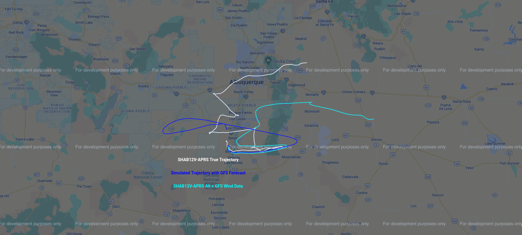
main.py runs as is against the bundled SHAB14-V example flight — a GFS
forecast plus the real SHAB14-V APRS track, so the prediction is overlaid on the
actual trajectory. (Point forecast["file"] at the bundled ERA5 file to run
the same flight off ERA5 instead.) From the parent directory: run
python3 -m EarthSHAB.main
You should see:
Altitude vs time plots
Temperature profiles
3D wind/atmosphere visualization
Interactive trajectory map (html file in /trajectories directory)
Note
New since version v1.1, main.py supports comparing simulations (using either a GFS forecast or ERA5 renalysis) to a historical balloon flight. At this time, only balloon trajectories in the aprs.fi format are supported. Flights using APRS devices for real time tracking can be downloaded after landing from APRS.fi. To use this functionality, change balloon_trajectory in the configuration file from None to a filename.
Configuration File
config.py is the central control file for all EarthSHAB simulations. In most cases, this is the only file you need to modify.
Many parameters can be adjusted for running EarthSHAB simulations and the parameters are grouped together into convienent categories:
balloon_properties: includes parameters for adjusting the balloon size and material propeties. Currently only the ‘sphere’ shape is supported. If using a standard 6 m charcoal-coated SHAB balloon, the payload and envelope masses are the only parameters that need to be updated.
netcdf_gfs: includes parameters for downloading and saving GFS netcdf forecasts from NOAA via
saveNETCDF.py. Currently only supporting forecasts with a resolution of 0.25 degrees for better trajectroy prediction accuracy.simulation:
forecast: Selects the forecast file to simulate against.
forecast["file"]points at a single v2-canonical netcdf in the forecasts directory; the source (GFS vs ERA5) is read automatically from the file’sinstitutionattribute, so there is no separate forecast-type switch.forecast["wind_interpolation"]chooses the wind interpolation method (see Wind Interpolation Methods).forecast[“forecast_update_interval”]: adjusts how often wind speeds are looked up (default is once per 60 seconds). The fastest look up rate is up to 1.0 s, which provides the highest fidelity predictions, but also takes significantly longer to run a simulation.
dt: is default to 1.0 s integrating intervals.
earth_properties: include mostly constant proeprties for earth. These values typically don’t need to be changed, however the ground emissivity and albedo might be changed if predicting balloon launches over oceans or snow covered locations.
Tip
If when increasing dt, NaNs are introduced, this is a numerical integration issue that can be solved by decreasing dt. Most values over 2.5 s cause this issue when running a simulation.
Other Examples
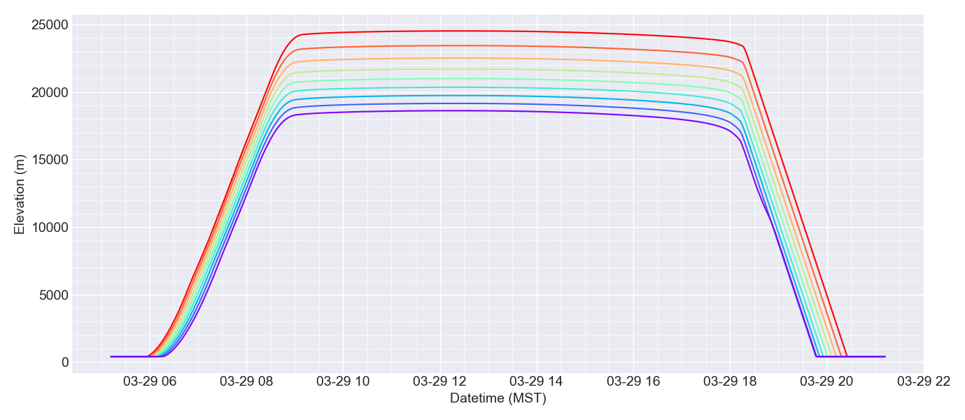
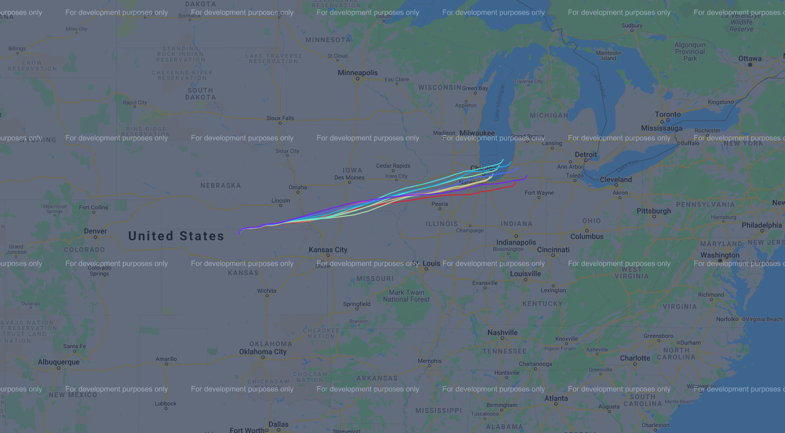
python3 -m EarthSHAB.predict uses EarthSHAB to generate a collection of altitude and trajectory predictions at different float altitudes. Estimating float altitudes for a standard charcoal SHAB balloon are challenging and can range from SHAB to SHAB even if all the balloon_properties are the same and the balloons are launches on the same day. This example produces a rainbow altitude plot and interactive google maps trajectory prediction. The float altitudes are adjusted by changing the payload mass in .25 increments to simulate varrying float altitudes.
python3 -m EarthSHAB.trapezoid provides a rough example of how to use EarthSHAB with a manual altitude profile to estimate wind-based trajectory predictions. Alternatively, you can generate a csv file in the aprs.fi format and inclue it in config.py.