Wind Interpolation Methods
EarthSHAB’s unified Forecast reader (which serves both GFS and ERA5 netcdf
files) interpolates wind from the discrete pressure levels of a forecast to the
balloon’s continuous altitude during simulation. The wind field is selected by
three orthogonal config fields:
# src/EarthSHAB/config.py
forecast = dict(
    file = "src/EarthSHAB/forecasts/gfs_0p25_3h_20220822_12.nc",  # GFS or ERA5 .nc
    wind_interpolation = 'linear_full',     # horizontal stencil + alt/time scheme (this page)
    advection          = 'geodesic',        # how wind displaces the balloon each step
    backend            = 'numpy',           # wind-lookup implementation tier
    ...
)
wind_interpolation— the horizontal stencil and the altitude/time interpolation scheme. Four methods, documented below:linear_neighbors/linear_full/spline_full/bilinear.advection— how the sampled wind moves the balloon:'geodesic'(default; WGS84 ellipsoid step, re-anchored at the balloon each step) or'tangent_plane'(spherical step about the fixed launch anchor). This changes the trajectory but not the wind lookup.backend— the wind-lookup implementation tier:'numpy'(default, float64, matches the historical scalar path bit-for-bit),'numba'(JIT batch kernels; only faster for batched/Monte-Carlo sampling, not single trajectories), or'xarray'(slow reference path). All three produce the same trajectory within float32-cache tolerance, sobackendis purely a speed/dependency choice, not a physics one.
The altitude/time interpolation math lives in
EarthSHAB.utils.wind_interp (the horizontal stencils and the
apply_* appliers); the data-access tiers live in
EarthSHAB.utils.forecast_backends. Forecast is a thin
orchestrator that selects a backend and a method and exposes
getNewCoord() /
getNewCoords(). The scalar
wind_alt_Interpolate2() entry point is kept
for API parity and routes through the selected backend, dispatched by
config.forecast['wind_interpolation'].
Methods
linear_neighbors (historical default)
For the two pressure levels straddling the query altitude, convert the sampled (u, v) winds to bearing + speed, then linearly interpolate the bearing and the speed between those two levels (with a 0/360° wrap correction so a wind shifting from 350° → 10° doesn’t sweep the long way around through 180°). The interpolated bearing/speed is then converted back to (u, v).
Pros: physically intuitive — speed and direction vary linearly. Matches a forecaster’s mental model of how wind changes with altitude.
Cons: the bearing → u/v conversion is non-linear, so the resulting u/v curve has subtle distortions near 0/360° crossings. Discards information from all the other pressure levels in the profile.
linear_full
Run numpy.interp independently on the u and v components
across the full altitude profile (all pressure levels at once), then sample
at the query altitude.
Pros: simple, fast, no angle-wrap edge cases — u and v are ordinary scalars. Empirically the best-performing method in the EarthSHAB benchmark suite (see Evaluation); the win comes from using the cartesian representation rather than from any fancier interpolation. Recommended as the new default.
Cons: in regions where two adjacent pressure levels have opposing winds (a true wind shear layer), linear u/v interpolation smears the bearing through 90° in a way that isn’t physically meaningful at intermediate altitudes — but the same smearing happens to the balloon in reality across a thin shear layer, so this is rarely a problem.
spline_full
Fit a scipy.interpolate.CubicSpline to u and v independently
across the full altitude profile, then sample at the query altitude.
The spline is built with extrapolate=False; for query altitudes
outside the sampled range (typically above the highest pressure
level — the balloon often flies higher than the top GFS level), the
method falls back to numpy.interp (which clamps to the endpoint)
rather than letting the spline extrapolate, since unconstrained cubic
extrapolation overshoots wildly at the boundaries.
The helper also dedupes the input altitude array before fitting,
because EarthSHAB.Forecast.Forecast.fill_missing_data() clamps the top
few NaN entries to the last valid altitude, producing duplicate h
values that CubicSpline cannot handle. If fewer than four unique
altitudes remain after dedup, the helper transparently falls back to
linear interpolation.
Pros: smooth derivatives — useful for visualization or for estimating wind shear (du/dh, dv/dh). Reproduces all sampled pressure-level winds exactly (within floating-point noise).
Cons: can introduce small unphysical oscillations between sparsely-sampled pressure levels. In the EarthSHAB benchmark, spline wins more individual launches than linear_neighbors but its mean landing error is slightly worse than linear_full — the launches it hurts, it hurts harder than the launches it helps.
bilinear
The other three methods snap to the single nearest lat/lon grid cell.
bilinear instead blends the (u, v, geopotential) columns across the
four surrounding cells with a bilinear weight, then applies the
linear_full altitude/time scheme to the blended column.
Pros: removes the horizontal “staircase” of nearest-cell sampling — wind varies smoothly as the balloon crosses grid-cell boundaries. Most noticeable on coarse grids (0.5°/1.0°).
Cons: four-cell reads instead of one. Near the forecast’s lat/lon edges the closed-form stencil (
numpy/numbabackends) extrapolates linearly where the nearest-cell methods clamp; thexarraybackend delegates toxarray.interp, which returns NaN just outside the grid rather than extrapolating.
When to pick which
For trajectory prediction, prefer
linear_full— it produced the lowest mean landing error in the 46-launch benchmark.For wind-shear analysis or visualization where smooth derivatives matter, use
spline_full.linear_neighborsis retained for bit-equivalent reproduction of pre-2026 EarthSHAB simulation results.bilinearis worth trying on coarse (0.5°/1.0°) grids where nearest-cell horizontal sampling is visibly blocky; on a 0.25° grid it usually differs little from the nearest-cell methods.
Visualizing the differences
The EarthSHAB.windmap.Windmap class exposes
EarthSHAB.windmap.Windmap.plotWindMethod() which renders the same
3D polar windrose used by EarthSHAB.windmap.Windmap.plotWind2()
and EarthSHAB.windmap.Windmap.plotWindVelocity() — radius =
altitude, angle = bearing, color = wind speed — but interpolates the
wind profile using one of the three production methods exactly as the
simulator would consume it. A companion helper,
EarthSHAB.windmap.Windmap.plotWindMethodsComparison(), composes
all three into one side-by-side figure with shared color and radial
scales.
Example:
from EarthSHAB.windmap import Windmap
import matplotlib.pyplot as plt

wm = Windmap()
wm.plotWindMethodsComparison(wm.hour_index, wm.LAT, wm.LON)
plt.show()
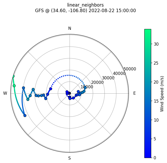
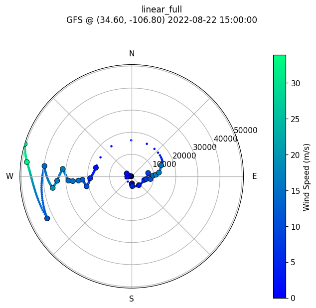
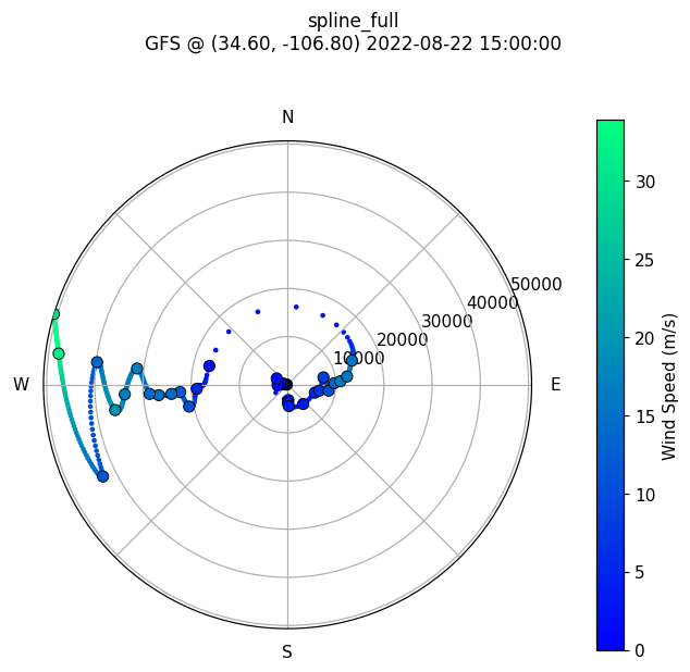
The three polar windroses below show the same GFS profile interpolated by each production method (large black-edged dots = raw pressure-level samples; small dots = the dense interpolated samples the simulator sees between pressure levels). Same color and radial scale across all three for direct comparison.
What to look for:
linear_neighbors produces piecewise-linear arcs between adjacent pressure-level samples (bearing and speed each interpolated linearly, with 0/360° wrap correction). Other pressure levels in the profile are not consulted.
linear_full interpolates u and v linearly across the whole profile. Near 0/360° crossovers the polar trace can take a longer arc than
linear_neighborsbecause cartesian u/v interpolation passes through the origin rather than around it — visible as the curve dipping toward the center between two opposing-wind samples.spline_full threads smoothly through every pressure-level sample but visibly overshoots between sparsely-spaced ones — look for radial wobbles where the small dots momentarily leave and re-enter the corridor between adjacent black-edged samples. This overshoot is what hurts spline’s mean landing error in the benchmark even though it wins more individual launches.
See also
Forecast — unified forecast reader API
windmap — windrose and hodograph plotting
Evaluation — batch evaluation comparing wind methods