Single Evaluation

A single evaluation runs one simulation against one historical balloon flight and reports how close the simulation came to the truth. It uses the current config_earth.py directly.

Useful for:

• Comparing an individual ground truth SHAB flight trajectory to the EarthSHAB model, with GFS or ERA5

• tuning single physical parameters (Upsilon, interpolation methods, emissivity, etc.)

For batch evaluating multiple flights and campaigns, see Batch Evaluation.

Prerequisites

Two required inputs must be in place before running the evaluation, with SHAB14V as an example:

1. A downloaded forecast file (GFS or ERA5) in src/EarthSHAB/forecasts/.

2. A balloon trajectory CSV in src/EarthSHAB/balloon_data/SHAB14V-APRS.csv.

Note

Trajectory CSVs can be downloaded after landing from APRS.fi and LightAPRS-W trajectory .csv formats are accepted. More coming soon. The trajectory loader auto-detects the format from the column header.

Configure config_earth.py

1. Point to your APRS trajectory file:

balloon_trajectory = parent_dir + "balloon_data/SHAB14V-APRS.csv"

2. Set the simulation start time to match launch:

start_time = datetime.fromisoformat("2022-08-22 14:36:00")  # UTC

3. Set the launch coordinates and ground elevation:

simulation = dict(
    start_time = start_time,
    sim_time = 15,        # hours — set 1–2 hours beyond actual flight duration
    start_coord = {
        "lat": 34.60,
        "lon": -106.80,
        "alt": 1000.,     # ground elevation (m), also used as min_alt
        "timestamp": start_time,
    },
    min_alt = 1000.,
    balloon_trajectory = balloon_trajectory,
    ...
)

4. Set balloon physical properties:

balloon_properties = dict(
    shape = 'sphere',
    d = 5.8,        # diameter (m)
    mp = 0.9,       # payload mass (kg)
    mEnv = 2.1,     # envelope mass (kg)
    ...
)

5. Select your forecast type and file:

forecast = dict(
    forecast_type = "GFS",   # or "ERA5"
    forecast_start_time = "2022-08-22 12:00:00",
    GFSrate = 60,
)

Run the Evaluation

From the repository root:

python -m evaluation.evaluate

The single evaluator does three steps:

1. Forward simulation — runs the full physics-based trajectory prediction using the provided forecast (same as main.py and predict.py)

2. Reforecast simulation — re-runs the same flight, but instead of using the simulated altitude profile, it forces the balloon onto the actual altitude profile and only uses the forecast for horizontal winds. This isolates wind error from vertical-motion error.

3. Cross-comparison metrics — phase detection, float statistics, landing distance, temperature/pressure MAE. and outputs a statistics table, multi-panel comparison PNG, and an interactive trajectory HTML.

Single Evaluation Output

Console report:

====================================================================
  EarthSHAB Evaluation: SHAB14V-APRS
====================================================================
  Metric                               Sim      Truth       Diff  Unit
--------------------------------------------------------------------
  Float Alt Mean (m)                 18988      20396      -1407  m
  Float Alt Std (m)                    378        447        -69  m
  Ascent Rate Mean (m/s)              1.91       2.36      -0.45  m/s
  Ascent Rate Std (m/s)               0.33       0.96      -0.63  m/s
  Descent Rate Mean (m/s)            -2.82      -2.37      -0.44  m/s
  Elapsed Time (min)                 779.8      789.0       -9.3  min
  Landing Lat (°)                  34.7816    34.5468     0.2347  °
  Landing Lon (°)                -106.7869  -109.1340     2.3471  °
--------------------------------------------------------------------
  Distance Off (m)                                        216697  m
  Landing Time (MST)  2022-08-22 20:35   2022-08-22 20:46  -11.2  min
--------------------------------------------------------------------
  Temperature MAE                                          38.55  K
  Pressure MAE                                               659  Pa
--------------------------------------------------------------------
  GFS Forecast + Truth Altitude (reforecast landing vs truth)
  Distance Off (m)                                         44811  m
====================================================================

Start-time analysis
Current config start_time : 2022-08-22 14:36:00 UTC
First APRS transmission   : 2022-08-22 14:37:53 UTC  (1557 m)
Estimated launch time     : 2022-08-22 14:32:23 UTC
Suggested start_time      : "2022-08-22 14:32:23"

Tip

The start-time analysis at the bottom takes the first ascending APRS points (v > 0.5 m/s), averages their vertical velocity, and linearly extrapolates the first APRS altitude back down to min_alt. If the suggested time differs significantly from your configured start_time, update config_earth.py and re-run. APRS trackers often miss the begining of ascent due to ground interference.

Comparison plot:

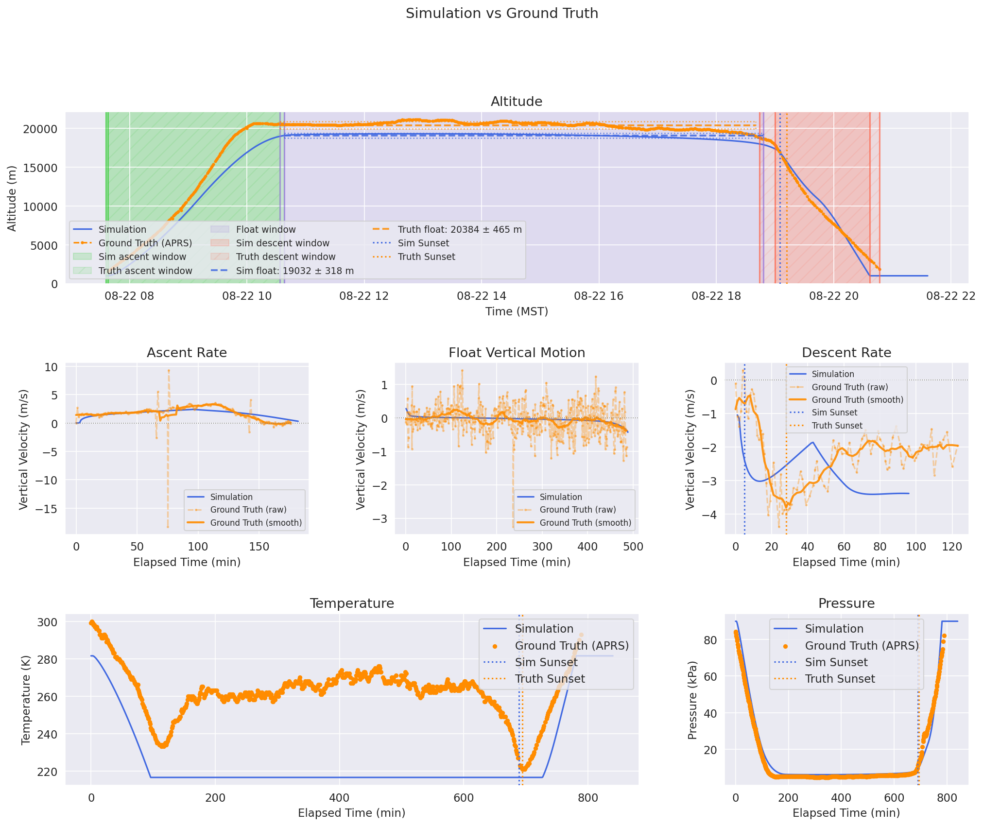
• Altitude Profile. EarthSHAB Simulated trajectory in blue, APRS ground truth in orange. Colored bounding boxesshow the detected phase windows for sim (solid fill) and truth (hatched fill):

  • green = ascent window

  • purple = float window

  • red = descent window

  The float-altitude estimate is overlaid as a horizontal mean line bracketed by ±1 σ rails. Sim sunset (blue dotted) and truth sunset (orange dotted) appear at the wall-clock instant the solar zenith first crosses 90° (refraction-adjusted) along each trajectory.

• Row 2 — Per-phase velocity windows. Three subplots zoomed to the ascent / float / descent phase respectively. Each subplot uses phase-aligned elapsed time on the x-axis so sim and truth align even when their wall-clock phase boundaries do not match. Truth velocity is drawn twice: faded markers for the raw finite-difference signal and a solid line for the rolling-mean smoothed version.

• Row 3 — Temperature and Pressure. Sim T_atm vs onboard sensor; sim altitude → ISA pressure vs onboard barometer. X-axis is elapsed time for both traces, allowing visual comparison even if launch wall-clock times differ slightly.

Saved files (written to evaluation/):

File	Contents
<stem>.csv	All metrics in tabular form (Sim, Truth, Diff)
<stem>.png	Three-row comparison figure shown above
EVALUATION_<stem>.html	Interactive trajectory map (Google Maps): simulated trajectory, reforecast trajectory, and APRS ground-truth track on a single map

The filename stem is built from the trajectory name, forecast type, and launch date — e.g. SHAB14V-APRS_GFS_2022_8_22.

Calculations and Assumptions

Phase detection (ascent / float / descent)

Implemented in _detect_phases().

The detector runs the same algorithm against both the simulation and the truth trajectory. The goal is a robust three-way segmentation that survives noisy APRS data and survives “no float” trajectories where the balloon peaks and immediately falls.

Step 1 — locate the high-altitude region

The maximum altitude is taken with np.nanmax (so a single dropped APRS altitude reading does not collapse the detector). Indices where alt ≥ 0.90 · max_alt define the high-altitude bracket [i_enter, i_exit]. NaN altitudes evaluate False and are naturally excluded. If no point qualifies, i_enter = i_exit = argmax(alt).

Step 2 — find the float window inside the bracket

The vertical velocity is smoothed with a centred rolling mean. Window size is max(10, min(span // 6, 600)) where span = i_exit − i_enter, so it adapts to the length of the high-altitude region but is capped to avoid trivial smoothing on long flights.

The candidate float mask is |rolling-mean v| < v_float (default v_float = 1.0 m/s). Of all contiguous True blocks, the largest is chosen. It is then rejected if it is shorter than max(10, span // 4) — this rejects spurious float detections caused by the velocity zero-crossing at the apex of a “straight up, straight down” trajectory.

Step 3 — trim the float window

Even after thresholding, the start of the candidate block contains the deceleration into float (rolling mean still > 0.3 m/s) and the end contains the rapid descent out of float (rolling mean < −0.5 m/s). The block is trimmed inward until the rolling mean satisfies these tighter bounds. If trimming destroys the block (length < min_len), the float is discarded.

Step 4 — ascent and descent

Ascent and descent masks live strictly outside the high-altitude bracket to keep them clear of the curved transition regions:

• ascent_mask  = (v > v_linear) & (i < i_enter)

• descent_mask = (v < −v_linear) & (i ≥ i_exit)

v_linear defaults to 1.0 m/s.

Launch-type-aware behaviour

EarthSHAB only physically models a self-ascending solar balloon. When the launch_type field on a launch entry is set to something other than "standard", the evaluator alters phase detection and metric reporting so non-physical comparisons don’t pollute the results. The behaviour is identical between single and batch evaluations.

• "standard" (default) — full ascent / float / descent metrics.

• "helium_augmented" — ascent is helium-driven, faster than solar. Both sim and truth ascent masks are zeroed out, so Ascent Rate Mean / Std and Time to Float report N/A. Float and descent metrics remain valid and are scored.

• "grand_slam" — SHAB is carried by a separate weather balloon and released above its natural float altitude. Two changes:

  • Ascent metrics are zeroed (same as helium-augmented).

  • The float-search bracket is widened from alt ≥ 0.90 · max_alt to the entire post-apex region of the trajectory. Without this the detector clips to the brief weather-balloon release peak and misses the actual SHAB float plateau that follows the descent. The descent mask then begins at last_float_index + 1.

A row’s Type cell in Batch Summary Table shows which behaviour was applied; missing field is treated as standard.

Note

The forward simulation is unchanged — EarthSHAB still simulates a solar balloon ascending from min_alt regardless of launch_type. The flag only affects which phases of the observed trajectory get scored.

Truth-velocity smoothing

Before phase detection, the truth velocity is passed through a 5-sample centred rolling median (min_periods=1). The unsmoothed (raw) velocity is shown as faded markers. The smoothed version (solid line) is used in the phase detector and the truth ascent/descent rate metrics.

NaN handling

• Phase detection: np.nanmax and np.nanargmax for altitude; alt >= threshold evaluates False on NaN, so NaN points cannot leak into the high-altitude bracket.

• Trajectory map: _drop_nan_coords filters any (lat, lon) pair where either coordinate is NaN before the polyline is drawn. This stops gmplot from drawing a line through (0, 0).

Altitude “Reforecast” (truth altitude profile + forecasted wind)

The reforecast landing distance removes the vertical-motion error, showing the balloon trajectory had it flown the exact altitude profile but in the forecast wind field.

1. The forecast is queried at each trajectory point (time, lat, lon, alt) to get the forecasted wind vector (u, v) that would have acted on the balloon at that instant.

2. The wind is integrated forward in time using the ground-truth altitude profile (no buoyancy, no envelope dynamics), producing a reforecasted trajectory.

Onboard temperature & pressure

• Temperature MAE — the simulated atmospheric temperature T_atm is linearly interpolated to each APRS timestamp and compared against the parsed onboard temperature, in kelvin.

• Pressure MAE — the ISA-1976 pressure model is evaluated at each APRS altitude and compared against the parsed onboard barometer reading, in pascals. This is a sanity check on the APRS pressure sensor and on the altitude estimate, not on the simulator.

Both metrics report N/A if no parseable readings exist.

Sunset detection

Sunset for sim and truth is computed independently:

• Sim sunset: scans every 60 sim steps; converts local time to UTC using the configured GMT offset and tests solar_zenith_adjusted(t_utc, lat, lon, alt) ≥ π/2. The first crossing is the sunset.

• Truth sunset: same test, but using each APRS row’s actual lat/lon/altitude and the row timestamp. Crucially, the APRS dataframe is sorted by time first because aprs.fi exports are newest-first by default. No model data is used for this calculation.

Both crossings are drawn on the altitude / velocity / temperature / pressure panels so you can visually correlate sunset cooling with descent onset.

Note

Sunset times can differ significantly between sim and truth, even on the same flight, because of differences in the simulated vs ground truth horizontal trajectory. This is a good example of how vertical-motion error can cause a balloon to experience a different wind field and therefore a different sunset time, which in turn affects the descent onset and landing location.